What you may miss about the core concept of the GAN model. Here is what I learnt from my dissertation.

Photo by Alina Grubnyak on Unsplash

And it is time of the year. I have completed my dissertation and officially received a Master’s degree with distinction. However, I want to write this blog to summarize what I found after researching during the summer semester.

Firstly, I have to introduce my research topic.

SE-GAN: Sentiment-Enhanced GAN for Stock Price Forecasting-A Comprehensive Analysis of Short-Term Prediction

It looks like a long title. Anyway, I will briefly overview my project in the figure below.

Fig. 1. SE-GAN architecture. Photo by Author

I used Microsoft stock data from the EIKON database of LSEG and historical stock indexes, such as the S&P 500, Dow Jones, etc., from Yahoo Finance incorporated into sentiment scores from the Microsoft headlines.

Fig. 2. Sentiment analysis pipeline of Microsoft stock headlines. Photo by Author

I used FINBERT (an existing pre-trained model specifically for financial data) for sentiment analysis. After getting the final dataset, it was trained using the GAN model.

Some people may know GAN (Generative Adversarial Network) as a generative architecture for image generation, and I used it as a predictive model. How does it work?

Before that, let's go back to the concept of the GAN model. The GAN model sounds like an approach to train the model rather than the model itself. How?

Fig. 3. Generative Adversarial Network Architecture. Photo by Author

GANs are comprised of two models: Generator and Discriminator. The generator generates data, and the discriminator discriminates/judges the correctness of the input data.

The generator model and the discriminator can use any model. As such, I used GRU (Gated Recurrent Unit) as a generator model with a linear activation to predict the continuous value (closing price) and MLP (Multilayer Perceptron) as a discriminator with a sigmoid function to predict the probability of input data belonging to two categories (fake or real).

GRU model

Input → GRU (50) (return_sequence=True) → Dropout (dropout rate=0.2) → GRU (50) (return_sequence=False) → Dropout (dropout rate=0.2) → Dense (1)

MLP model

Input →Dense (256) → LeakyReLU (α = 0.2) → Batch Normalization → Dense (128) → LeakyReLU (α = 0.2) → Batch Normalization → Dense (64) → LeakyReLU (α = 0.2) → Batch Normalization →Dense (1),Sigmoid

My generator model generated the closing price, while the discriminator differentiated between the predicted and real prices. The generator received feedback from the discriminator to refine the generator’s ability by predicting the closing price as close to the real price to beat the discriminator. On the other hand, the discriminator had to identify the fake closing prices from the real ones. To make it simple, it is a competitive approach between two models. So, this is the objective function of the GAN model.

The objective function of the GAN model

min_G max_D V (G, D) = E[log D(X_real)] + E[log(1 −D(G(X )))]

min_G max_D V (G, D) = E[log D(X_real)] + E[log(1 −D(X_fake))]

Minimizing generator loss and maximizing discriminator loss.

Some people may be confused about the generator model. How is it reliable to use fake data to predict the stock price?

It needs to go to the core concept of the GAN model to make it clearer. The core concept of the GAN model is “Adversarial”; due to its name, “Generator”, people are confused. Apart from that, there is a nuance between the “Generative” and the “Predictive” models.

To answer the question and clarify, the model for this research acts as an adversarial network specifically used for predictive problems.

And I will explain why.

During my research, I reviewed previous research literature. I found a difference between the original GAN model (image generation) and the research using this model in other areas (stock price forecasting or time series forecasting).

This is the original code for image generation.

@tf.function
def train_step(images):
    noise = tf.random.normal([BATCH_SIZE, noise_dim])

    with tf.GradientTape() as gen_tape, tf.GradientTape() as disc_tape:
      generated_images = generator(noise, training=True)

      real_output = discriminator(images, training=True)
      fake_output = discriminator(generated_images, training=True)

      gen_loss = generator_loss(fake_output)
      disc_loss = discriminator_loss(real_output, fake_output)

    gradients_of_generator = gen_tape.gradient(gen_loss, generator.trainable_variables)
    gradients_of_discriminator = disc_tape.gradient(disc_loss, discriminator.trainable_variables)

    generator_optimizer.apply_gradients(zip(gradients_of_generator, generator.trainable_variables))
    discriminator_optimizer.apply_gradients(zip(gradients_of_discriminator, discriminator.trainable_variables))

This is the code using GAN for stock forecasting. (From the paper “Stock price prediction using Generative Adversarial Networks” [1])

 @tf.function
    def train_step(self, real_x, real_y, yc):
        with tf.GradientTape() as gen_tape, tf.GradientTape() as disc_tape:
            generated_data = self.generator(real_x, training=True)
            generated_data_reshape = tf.reshape(generated_data, [generated_data.shape[0], generated_data.shape[1], 1])
            d_fake_input = tf.concat([tf.cast(generated_data_reshape, tf.float64), yc], axis=1)
            real_y_reshape = tf.reshape(real_y, [real_y.shape[0], real_y.shape[1], 1])
            d_real_input = tf.concat([real_y_reshape, yc], axis=1)

            real_output = self.discriminator(d_real_input, training=True)
            fake_output = self.discriminator(d_fake_input, training=True)

            gen_loss = self.generator_loss(fake_output)
            disc_loss = self.discriminator_loss(real_output, fake_output)

        gradients_of_generator = gen_tape.gradient(gen_loss, self.generator.trainable_variables)
        gradients_of_discriminator = disc_tape.gradient(disc_loss, self.discriminator.trainable_variables)

        self.generator_optimizer.apply_gradients(zip(gradients_of_generator, self.generator.trainable_variables))
        self.discriminator_optimizer.apply_gradients(
            zip(gradients_of_discriminator, self.discriminator.trainable_variables))
        return real_y, generated_data, {'d_loss': disc_loss, 'g_loss': gen_loss}

The difference between these two code blocks is that the original code uses random noise data as the initial data for training the generator model.

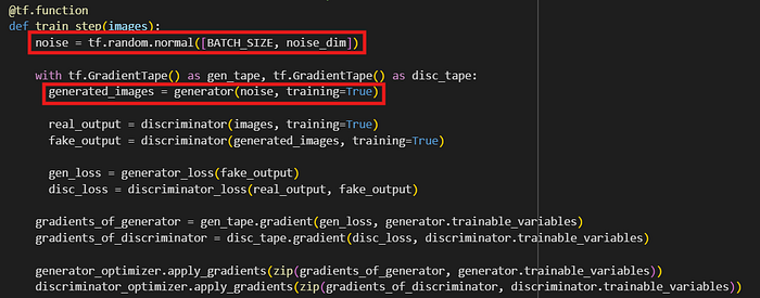
In contrast, the second block uses the real training data, in this case, other features, such as HIGH, LOW, OPEN, and COUNT, except the closing price (CLOSE) since the model will forecast later, as the initial input.

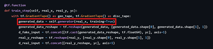
For this reason, the generator model for stock forecasting acts as a model to predict the closing price of the next date from the stock data of previous dates. In contrast, the generator model for image generation employs a random matrix as an input, and attempts to generate an output close to the real output without having a foundation knowledge or existing features from the real images fed to the model as the initial point.

Fig.4. The loss of GAN model for training sequence length of 30 days of input data. Photo by Author

As mentioned above, the GAN model is a competition between two models to achieve their objective function (minimizing generator loss and maximizing discriminator loss). The generator has to predict/generate the output to fool the discriminator, while the discriminator must not be fooled by its opponent. Therefore, it can expand to a broad range of implementations.

I wrote this blog post mainly because I will shift my research interest from time series forecasting to another research area. I want to leave what I have studied so far for further review.

I have uploaded my code, report, and presentation at the end of my blog in this repository. You can take a look at it.

Thank you for reading.

REFERENCE

[1] H. Lin, C. Chen, G. Huang, and A. Jafari, “Stock price prediction using Generative Adversarial Networks”, Journal of Computer Science, vol. 17, no. 3, pp. 188–196, 2021.